Computational Textual Analysis: Is it literature?

Is there a definitive definition for literature? I was thinking to myself about this the other day, and decided to find out. Before I set out on this experiment I'll make it clear that I think the answer is very subjective, and that although there are aspects found within most books that are considered true literature, these are not found within all of them. The initial list of books that I considered literature (with which to train my software) are widely spread in terms of theme, publication date and writing style, but the key point is they are chosen, therefore a concept of literature already exists in the person who chooses a list. The program I set out to write would be able to determine whether or not any piece of text was (or wasn't) literature by matching the similarity of various features of a piece of text, to this concept of true literature. It should also be noted that the program is language independent.

I'll start by explaining briefly some of the characteristics that I decided to use in order to measure the level of literature in a piece of text:

• Sentence length
• Average word length
• Unique words
• Vocabulary Score (unique words / total words)
• Vocabulary Deviation
• Character Deviation
• Word Entropy
• Character Entropy

Sentence length and word length were calculated by splitting the text into components with the splitting parameter for sentences being a full stop, and for words being a space. Note that words can therefore include punctuation; "this" classes as a different word to "this." when it is at the end of a sentence. This gives us some information about where words are used in sentences.

Unique words are simply words without repeats, for example in the text chunk "hi hi there there there", the unique words are "hi" and "there". These can be used to provide what I've called a vocabulary score. The vocabulary score essentially allows us to create a measure of the range of words used, that is (almost) independent of the length of the text. I say almost, because the range of vocabulary in the English language is limited, therefore as text chunks become longer (for example in a very long novel such as War and Peace) the vocabulary score will automatically decrease.

The vocabulary and character deviation involve counting the number of repeats of each word and character - then calculating the standard deviation of this data set. The former is a good measure of how comfortable an author is using a wide range of words, as opposed to using them occasionally.

Finally two very important measures of "literaryness" are the entropy of words and characters. During initial experiments I found that these tend to stay fairly constant for the "literature" used for training. To calculate the entropy of a set the following calculation is used:

Entropy = - SUM [ Ki log2 ( Ki ) ],

where Ki is the probability of a member of the set (in this case a word or character) occurring.

The next step of the experiment was to find a transform of the values of the above features that yielded very similar results for all of my training set.

The following set of books were used in the training set:

• Franz Kafka, Metamorphosis
• Oscar Wilde, The Picture of Dorian Gray
• Sir Arthur Conan Doyle, The Hound of the Baskervilles
• Joseph Conrad, Heart of Darkness
• Jules Verne, Around the World in 80 Days
• J.D. Salinger, Catcher in the Rye
• Anthony Burgess, A Clockwork Orange
• Bram Stoker, Dracula
• George Orwell, Down and Out in Paris and London

And a value, which we'll call L was determined to be the smallest deviating transform of the textual features where:

L = (Word entropy + Character entropy - Word length) / Vocabulary score

Other features were found to range too much between the works.

Given an average L value the distance away from the mean was used to give any test text a literature score. Unfortunately this blog did not receive the title of literature, but then nor did Harry Potter and the Philosophers Stone, or Twilight, or a Mills and Boon title, A Fool For Love, so it seems to work quite nicely. 

A book I would consider to be literature, not on the training set was Kidnapped by Robert Louis Stevenson, and it did indeed score highly on the literature front which means the system works!

Below is the application, just click to launch it and post a comment with any results you might find:

Currently the results are a bit spurious, mostly because thresholds are fiddly to get right, but with a bit of work and some other parameters I have been thinking about, this kind of textual analysis really might help us spot the next classics! The program currently works best with whole books, there are a load of free eBooks that are now in the public domain which you can test the software with!

2D Dynamic Shadow Casting (and Lighting)

After having a little think about how to do this effectively, the answer was actually rather simple (which ins't entirely in keeping with the rest of this blog).  My previous attempts involved raytracing the 2D scene. By stepping through every single point in the scene, and calculating the path to it from the light source a per pixel map of brightness can be generated. I decided however that this was far to CPU intensive for high complexity scenes so went down a simpler route. The basic algorithm was:

• Trace a path from the light source to each vertex in each shape,
• Continue these paths outwards from the shape, thus casting a shadow
• Generate polygons to be filled in the shadow colour with pairs of these paths
• Draw a light mask (just a circle with a transparency gradient over the floor)

Just click the first image to launch the experiment. I am quite pleased with the results!

The image below shows the intermediary path tracing step:

By changing the light source mask a directional torch like effect is simple to reproduce, again just click to launch the app:

Colour Palette Creator

I am sure that there are hundreds of tools like this on the web, but I thought it would be quite interesting to produce a colour palette based on an image. Imaging you are designing a website and you really like the colours used in a particular piece of art, then you've come to the right place. This software will extract the most common colours in an image, and also give you the average colour.

The method used to calculate these is very simple. To calculate the average colour, simply sum all the RGB components of each pixel and divide by the total number of pixels. I do this using bitwise operators where:

R = HEX >> 16 & 0xFF
G = HEX >> 8 & 0xFF
B = HEX & 0xFF

and HEX = (R<<16 | G<<8 | B), useful stuff!

To calculate the palette I create an accumulator array which counts the number of each colour in the image. Before using this I reduce the number of colours in the image using some simple math.

I hope you find it quite interesting to have a play around with, just click the image to launch it. You can load your own images from your local computer to play around with it.

Real Time Feature Point Tracking in AS3

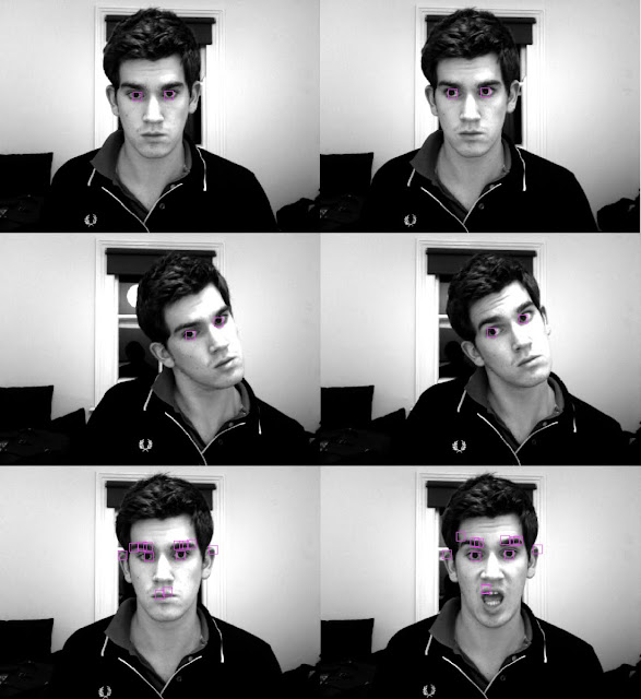
Its a bit late, so instead of posting a long informative post about how feature point tracking works I thought I'd just upload some of my results from this evening. I think its quite exciting stuff. The image shows feature point tracking working relatively well on my pupils, and also on other facial features (the last two images). I am very pleased with the result.

A related project I have also been working on this evening is optical flow which I am close to getting 

working, here is a preview of what is to come:

Both methods are used in tracking objects in moving images and have been implemented in real time. I will post sample movies and some explanations shortly so you can play around with them yourself.

Computer Vision: Regional Differencing

I have always been very excited by the idea of computer vision. At the same time I find the concept of teaching a computer to sift through a grid of pixels, whilst gaining some sort of an insight into their meaning quite astounding. When we as humans look at a scene we can immediately identify objects of interest to us. We look at a boat and immediately can tell that it is a boat and not for example a chair. We can do this, even if we have never seen that particular boat before. Computers struggle with this kind of visual finesse, although there are examples (see Assimo) that are already performing very well.

Back to the point: I was looking at this situation and thought to myself that humans find it incredibly easy to establish important features in any image. Take for example the image to the left, we can see clearly the line where the water meets land at the far edge of the lake, we can see trees, we can see a ridge and its reflection, and we can see clouds. These geometries are made visible to use because of contrast and colour differences between regions in the image. I decided to think of a way for a computer to do this. I'm sure the method has been done before under a different name, but I couldn't find any material on it so I've decided to call the method "Regional Differencing".

The method is fairly simple, but I am happy with the results. First the image is split into square regions of a constant size. The colour of these regions is equal to the average colour of the pixels contained within it. The result of this is a kind of pixilation as can be seen in the picture to the right. Now taking the colour values of every single pixel in the previous image, we can compare the value to that of the average regional colour.

The result of this is quite interesting because areas that don't fit in with their surroundings are clearly distinguishable in the image. In this article I'd like to argue that this is part of the reason why humans are so good at picking out the geometries mentioned above. Humans can happily distinguish between different regions, even where differences are relatively subtle. Combining this ability with memory of collections of shapes, we can identify objects very successfully.

So lets take a look at some of the results (as always click the first one to launch the application and try it out yourself):

The above 3 images show three different threshold levels for a constant pixel size, but if you run the app yourself you can also vary the pixel size yielding interesting results. At high thresholds it is interesting that the first objects that are made out are the trees and the line at the end of the lake, whereas the last objects made out are the clouds. Looking back I wonder if I found myself looking at these points before anything else.

There are many other ways to produced these kinds of data, including the Sobel operator method shown in various previous posts but sometimes it is nice to take a new approach.

Regional Growth Segmentation: Superpixels

I recently came across some impressive software from some researchers at Stanford University (who else), called Make3D which takes any 2 dimensional images - preferably outdoor images, and converts them into 3D models. The whole 2D to 3D process begins with a method called image segmentation, where structures in an image are separated into superpixels. Superpixels are collections of pixels with similar properties - for example saturation, colour, brightness etc.

I decided to write some software capable of creating the superpixel structure, and segmenting an image. The route I went down is called regional growth segmentation. Superpixels grow outwards from a sample pixel, and depending on the similarity of tested pixels to the superpixels, they are either added to the superpixel, or create new superpixels...

Here are a few results with different thresholds for similarity (again, just click the first image to launch the application).

I'll take a look at some of the Make3D source code to see if I can generate some 3D planes from my superpixel, so stay tuned!

Generating Normal Maps: 2D Images

The normal map used in the previous post was generated from a 3D model, so calculating normals was quite trivial. Taking any two dimensional image and calculating accurate realistic normals on the other hand is not. I have used a simple method using Sobel operators which seems to work quite well.

The Sobel operator provides X or Y gradient information about a certain image. Lets take a look at an example (Picture courtesy of my lovely girlfriend Camilla). The picture below shows a 2D image, with no 3D data whatsoever.

The sobel operator works by calculating the gradient of an image based on a range of pixels surrounding the pixel being tested.

First the image must be turned into a greyscale image, so that only brightness values are taken into account. Then a sobal operator is applied in the vertical and horizontal direction.

The results of applying the sobel operators can be seen in these two images. With the horizontal and vertical sobel operators respectively. These images correspond to the red and green channels in the final image. Since we have no sensible way of calculating a bump map for the two dimensional image the blue channel will just be set to a maximum throughout the image.

Finally we can apply this to the 2D Deferred Normal Lighting simulation I wrote about in the last post. The effects are quite impressive, creating a distinctly 3D look from a 2D image (Just click the image to launch the application):

To expand on this slightly further I thought it would be interesting to apply this to a webcam stream. This meant calculating a normal map every frame on top of the per pixel lighting so the resulting application is quite CPU intensive. I'm not quite as pleased with the effects as previously as there seems to be a lot of noise in the image. It might work better for you guys, just click the next image to launch it:

2D Deferred Normal Lighting

Continuing on the same lines as my previous post I thought I would create a few more 2 dimensional lighting simulations. With a little help from a post on normal mapping from a post on Planet Pixel Emporium I was able to create some real time 2D deferred normal lighting using actionscript. The simulation works on a per pixel basis so for large images the method would get very slow.

First lets take a look at the final result and then I will explain how it works. Click the image to the left to start up the application. You'll notice that moving your mouse around over the image moves the light source. Not only does this change information about how far the light should spread, but also the direction of the light with respect to every pixel on the screen.

This allows images to be rendered with a far more realistic depth and 3D feel (compare it to the original image on the right). For this reason the method is  used in many modern computer games.

The effect is created using a normal map. A normal map is a way of encoding data about the orientation of a plane using RGB colour. The red channel in the image represents the horizontal gradient of a face, the blue channel represents the vertical gradient, and the blue channel represents the height data (a bump map). The image below shows the normal map used for the image. I created the application by calculating the dot product of the normal at each point in the image with the light vector shining onto that pixel from the mouse's location.

The greater the dot product the more direct the light shining onto a point. In addition to this a distance falloff is used for the light to create the torch-like effect. I just use a factor of one over the square root of the distance as my falloff.

Obviously what isn't being considered in this is shadow casting so it isn't quite a real ray trace, but using bump map information it would be possible to create a real time semi 2-d ray trace.

Just for fun here is another sample, just click to launch it:

2D Dynamic Lighting - well almost

I had a nice idea to create a 2D dynamic lighting experiment, where various light sources could be moved round and cast shadows in real time. I got started on the experiment and created a class to hold a coloured light source and then I got a little too excited by some of the pretty generative artwork I was making and decided to change the purpose of the experiment. I'll briefly explain how the light sources work. A light source is made up of a point, a colour and a falloff rate. By measuring the distance from each light source in an image, and summing the light values at those points it is simple to calculate the light intensity at each point in the image. Here are some results (just click to run the app):

Some of the effects remind me of binary star systems. Here are 2 more apps showing real time moving light sources with various effects:

Circle Packing - brute force approach

Earlier this year, as part of my degree, I carried out a project that involved measuring the fractal dimension, and packing densities of various systems. I thought I'd have a play around with something along similar lines, circle packing.

There are many subtle and interesting and above all intelligent ways of packing circles into spaces, but this is not one of them. I decided to take a brute force approach. This is the structure my algorithm took:

• Pick a random point, if it is within any circles that already exist find a new point
• Increase the radius of that point until it overlaps with either the edge of the scene, or another circle on the scene.
• Draw the circle

This is as far as I can tell, both the simplest approach and the slowest. Lets take a look at the results, click the image to run the application. An interesting idea is to draw a line between each circle when they collide. This forms a kind of node based structure between circles, creating a network where larger circles hold more power in the network. I wonder if you could create a page ranking system based on something like this...?

Benoit Mandelbrot - Fractals and the art of roughness

A personal hero of mine talks about fractals.



I enjoyed his quote at the end and found it quite relevant to a lot of the work I do on this blog:

"Bottomless wonders spring from simple rules... repeated without end"

Computer Vision and the Hough Transform

I was working on computer vision yesterday and went to my girlfriend's graduation ceremony today so haven't had a chance to upload. I decided to take another look at computer vision - and in this case a slightly more intelligent one than previously. The method I took a look at is known as the Hough transform. I think that the simplest and most effective way to explain how the Hough Transform works is using a bullet pointed list, but before I begin you should know that it is used to extract information about shape features from an image. In this case a line / all the lines present in an image.

• We start with an image in which we want to detect lines:

• First of all apply a Canny Line Detector to the image isolating edge pixels:

• At this stage, to reduce computation required in the next stage I decided to sample edge pixels instead of using all of them. The results for s=0.2 and s=0.9 are shown below:

• Then, for every possible pair of sampled edge pixels, calculate the angle of the line between it, as well as the distance to the origin. Plot a cumulative bitmap graph of angle against distance. The way I did this was to increase the pixel value in that location each time a distance/angle occurred. Recall that a line can be defined by an angle and distance to an origin. The resulting bitmap is known as the Hough Transform:

• By increasing contrast and playing around with thresholds in the Hough transform it is clear that 8 distinct regions are visible, we know that the detector has done its job as there are 8 lines in the original image:

• Remember that each point provides us with data about the line angle and distance from the origin, so lets use the flash API to draw some lines:

• As you can see the result isn't too bad at all, we get 8 lines, although they are a bit diffuse. The next step is to look into grouping algorithms to only pick single pixel points from the final hough transforms for each lines. In this version of the program a line is drawn for each pixel, which results in an angle and position range for each line. Pretty close though.

So thats how a Hough transform works for line detection. Just for fun, heres a real time hough transform on a webcam stream. Just click the image below to launch it.